Combine data: Forced choice + Free Choice (Dual Response Data)

[cybey]

Hello, everyone,

I am currently working on Dual-Response-None and would like to benefit from your experiences, especially how you did the estimation.
In my case, it is about a product that really everyone has and I know the characteristics of each respondent’s product, i.e. I can describe the product with my CBC attributes. Therefore, the None-Option corresponds to "stay with my current product". For example, corresponding forced and free choice sets look like this:

Forced choice set, task 1:


Free choice set, task 1:


In the free choice set, I assume that the change from the current product to an alternative is associated with disutility, which I take into account with an alternative specific constant (ASC).

Now I see two options to include the none-option in the estimates.

Option 1: Separate models
First, I estimate the model with only forced choice sets, then the one with free choice sets. In the second model, alternative 1 is the preferred option from the free choice sets, alternative 2 always the current product.
In my case, in model 2, the price is much more important than in model 1, and as expected, staying with the current product has a positive utility. The advantages I see are the easy estimation and parameter comparability. The disadvantages are that I have to separate models and I wonder which of these “the right model” is. This of course raises the question of whether there is THE right model, or whether the answers to the two data sets (forced choice vs. free choice) are comparable at all, since they are the result of different cognitive processes.

Option 2: Joint estimation
As with RP and SP data, I thought of an integrated estimation (as in Apollo example 22) using apollo_combineModels().
The advantage is that I get parameter estimators once and not separate for each model. The RLH value is slightly above that of model 1 (forced choice model), but far below model 2 (free choice model). More precisely:

Model 1: RLH ~0.69
Model 2: RLH ~0.82
Model 1+2 (combined): RLH ~0.71

Now I ask myself: What is the right way? Option 1 or 2? Or option 3, which is...?

I would like to hear about your experiences with the None-Option or Dual Response, if you have any. At Sawtooth the integrated estimation with Dual Response is usually considered superior. I'm not so sure that this is always true, though.

Best wishes
Nico

[stephanehess]

Nico

thanks.

First of all, I don't think it makes sense to compare the fit between the free and forced choice makes sense, whether you use a reliable measure or the unreliable RLH. The differences will just reflect the fact that your choice shares in the free choice are likely much more one-sided, i.e. their current product is chosen more often and the ASC captures this.

In a forced choice like this, the fact that one alternative is free (am I right in assuming that?) will really impact your cost coefficient.

The thing to do is to contrast two separate models to a joint model, but do so using robust measures, not RLH. Then you will see whether the choice process is indeed different, or whether you can merge the parameters.

Stephane

[cybey]

Hi Stephane,

Thanks for your advice.

In a forced choice like this, the fact that one alternative is free (am I right in assuming that?) will really impact your cost coefficient.

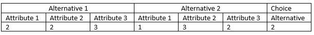
In the forced choice sets, respondents have to choose one of three (hypothetical) alternatives. None of these corresponds to the current product, nor do they contain alternative-specific constants (e.g. that alternative 1 is always a specific type of product, e.g. “train” instead of “car”). Thus, model 1 - the forced choice model - has one coefficient less than model 2 (the free choice model), which contains an alternative-specific constant for the current product. I could also omit the alternative-specific constant in model 2, since I can describe the current product of the respondents with my attributes and levels. However, I think that I would probably ignore the status quo effect by doing so.

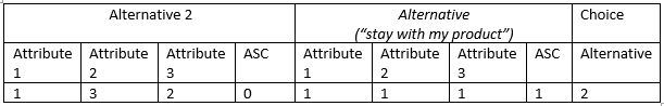
Furthermore, model 2 has only two alternatives, since the respondents only had to choose between the (hypothetical) new product chosen in model 1 and the current, old product. So it was just a situation where the survey participants were asked whether they would switch to this preferred alternative (yes/no). The number of observations is the same in both models, i.e. 12 choice sets per participant.

If I understand it correctly, in joint estimation, not all variables need to be present in both models, but they may differ in some. It is (only) important that the error terms of the two sub-models have an expected value of zero, i.e. it is actually important to insert the alternative-specific constant so that it incorporates the status quo effect.

I followed Apollo example 22 and estimated the joint model, both in preference space and in WTP space using Bayes estimation. SDR stands for "Separated Dual Response", i.e. this is model 2, and CBC is model 1.

Code: Select all

apollo_fixed = c("b_asc_2", "mu_SDR")

[...]

b_asc_1 = "N",
b_asc_2 = "F",
mu_CBC = "F",
mu_SDR = "F",

[...]

  hIW             = TRUE,
  priorVariance   = 1, 
  degreesOfFreedom = 30,

[...]

# Define settings for MNL model component
    mnl_settings = list(
      alternatives  = c(alt1=1, alt2=2, alt3=3),
      avail         = list(alt1=1, alt2=1, alt3=1),
      choiceVar     = Choice,
      V             = lapply(V, "*", mu_CBC),
      rows          = (ModelType=="CBC")
    )
    
    # Compute probabilities using MNL model
    P[['CBC']] = apollo_mnl(mnl_settings, functionality)
    
[...]

mnl_settings = list(
      alternatives  = c(alt1=1, alt2=2),
      avail         = list(alt1=1, alt2=1),
      choiceVar     = Choice,
      V             = lapply(V, "*", mu_SDR),
      rows          = (ModelType=="SDR")
    )

    # Compute probabilities using MNL model
    P[['SDR']] = apollo_mnl(mnl_settings, functionality)

    ### Combined model
    P = apollo_combineModels(P, apollo_inputs, functionality)

In both, preference space and WTP space, mu_CBC is < 1, at about 0.85.

After I had read the paper "Bradley, Daly (1997) - Estimation of Logit Choice Models Using Mixed Stated-Preference and Revealed-Preference Information", I made small changes regarding the alternative-specific constant.

Preference space:

Code: Select all

V[['alt1']] = b_asc_1_value + mu_SDR * ( b_Att1Lvl2_value * Att1Lvl2.1 + b_ Att1Lvl3_value * Att1Lvl3.1 + b_ Att2Lvl2_value * Att2Lvl2.1 + b_ Att2Lvl3_value * Att2Lvl3.1 + b_ Att2Lvl4_value * Att2Lvl4.1 + b_ Att3Lvl2_value * Att3Lvl2.1 + b_ Att3Lvl3_value * Att3Lvl3.1 + b_Price_value * Price.1)
V[['alt2']] = b_asc_2_value + mu_SDR * ( b_Att1Lvl2_value * Att1Lvl2.2 + b_ Att1Lvl3_value * Att1Lvl3.2 + b_ Att2Lvl2_value * Att2Lvl2.2 + b_ Att2Lvl3_value * Att2Lvl3.2 + b_ Att2Lvl4_value * Att2Lvl4.2 + b_ Att3Lvl2_value * Att3Lvl2.2 + b_ Att3Lvl3_value * Att3Lvl3.2 + b_Price_value * Price.2)
mnl_settings = list(
      alternatives  = c(alt1=1, alt2=2),
      avail         = list(alt1=1, alt2=1),
      choiceVar     = Choice,
      V             = V,
      rows          = (ModelType=="SDR")

WTP space:

Code: Select all

V[['alt1']] = b_Price_value * wtp_asc_1_value + b_Price_value * mu_SDR * ( wtp_asc_1_value + wtp_Att1Lvl2_value * Att1Lvl2.1 + wtp_ Att1Lvl3_value * Att1Lvl3.1 + wtp_ Att2Lvl2_value * Att2Lvl2.1 + wtp_ Att2Lvl3_value * Att2Lvl3.1 + wtp_ Att2Lvl4_value * Att2Lvl4.1 + wtp_ Att3Lvl2_value * Att3Lvl2.1 + wtp_ Att3Lvl3_value * Att3Lvl3.1 + Price.1)
V[['alt2']] = b_Price_value * wtp_asc_2_value + b_Price_value * mu_SDR * ( wtp_asc_2_value + wtp_Att1Lvl2_value * Att1Lvl2.2 + wtp_ Att1Lvl3_value * Att1Lvl3.2 + wtp_ Att2Lvl2_value * Att2Lvl2.2 + wtp_ Att2Lvl3_value * Att2Lvl3.2 + wtp_ Att2Lvl4_value * Att2Lvl4.2 + wtp_ Att3Lvl2_value * Att3Lvl2.2 + wtp_ Att3Lvl3_value * Att3Lvl3.2 + Price.2)    

In this case, only the common variables are scaled, but not the alternative-specific constant, which only exists in model 2. Here are the results:

Preference space:

Code: Select all

b_asc_2                          0.0000     NA
mu_CBC                           0.7782 0.0298
mu_SDR                           1.0000     NA

WTP space:

Code: Select all

wtp_asc_2                          0.0000     NA
mu_CBC                             0.7249 0.0325
mu_SDR                             1.0000     NA

The scaling parameter seems to be significantly different from 1. On the other hand, it is not a (simple) MNL model as in Apollo example 22 or described in the papers, but a MIXL model with Bayesian estimation. Nevertheless, even if I set hIW = FALSE and gFULLCV = FALSE, the parameter mu_CBC increases only slightly.

Kind regards
Nico

[stephanehess]

Nico

I would also include ASCs in the forced one as they may be choosing the options on the left more often, for example.

But your model is not identified - you're including the asc_1 in both alternatives, so it would cancel out. Of course, Bayesian estimation will give you a value for it, but it's not affecting the model. If you used classical estimation, you'd see this, but the newer versions of Apollo should also complain about it if you don't turn validation off

Stephane

[cybey]

Okay, I will, thanks for the tip.

The thing with the ASCs was just a typo (by copy and paste) in the forum entry. In the model, the values are correct, that is, ASC1 and ASC2 are specified correctly. The values of mu_CBC and mu_SDR are thus "correct", i.e. mu_CBC is <1.

Is there a rule of thumb as to when two data sets may be estimated as a joint model in the procedure described above? In the papers I have read so far (e.g. Bradley, Mark; Daly, Andrew (1997); Hensher, David A.; Bradley, Mark (1993)), no specific statements are made about this. The only advice they give: The closer to 1, the better.

Best wishes
Nico

[stephanehess]

Hi

I would always rely first on statistical tests, i.e. looking at whether the scale parameter is significantly different from 1, and also whether a joint model is not rejected by two separate models

Stephane

[cybey]

Okay, in my case the scale parameter is definitely different from 1:

Mean SD
mu_CBC 0.6887 0.0291
mu_SDR 1.0000 NA

The "CBC" is part of the survey with the forced choice sets, the "SDR" the part with the free choice sets.

How can I test, "[...] whether a joint model is not rejected by two separate models"? I suspect that simple statistical tests, e.g. wald test, do not work here? Or can the parameters simply be tested for significant differences?

[stephanehess]

Hi, regarding testing joint vs separate models, what you would do in classical estimation is a likelihood ratio test